
Dose-response across an antibody panel
Fit every titration in a binding assay and get back the curves that describe a real concentration-dependent response, with the rest named as background rather than quietly reported as potencies.
Start with the raw titrations
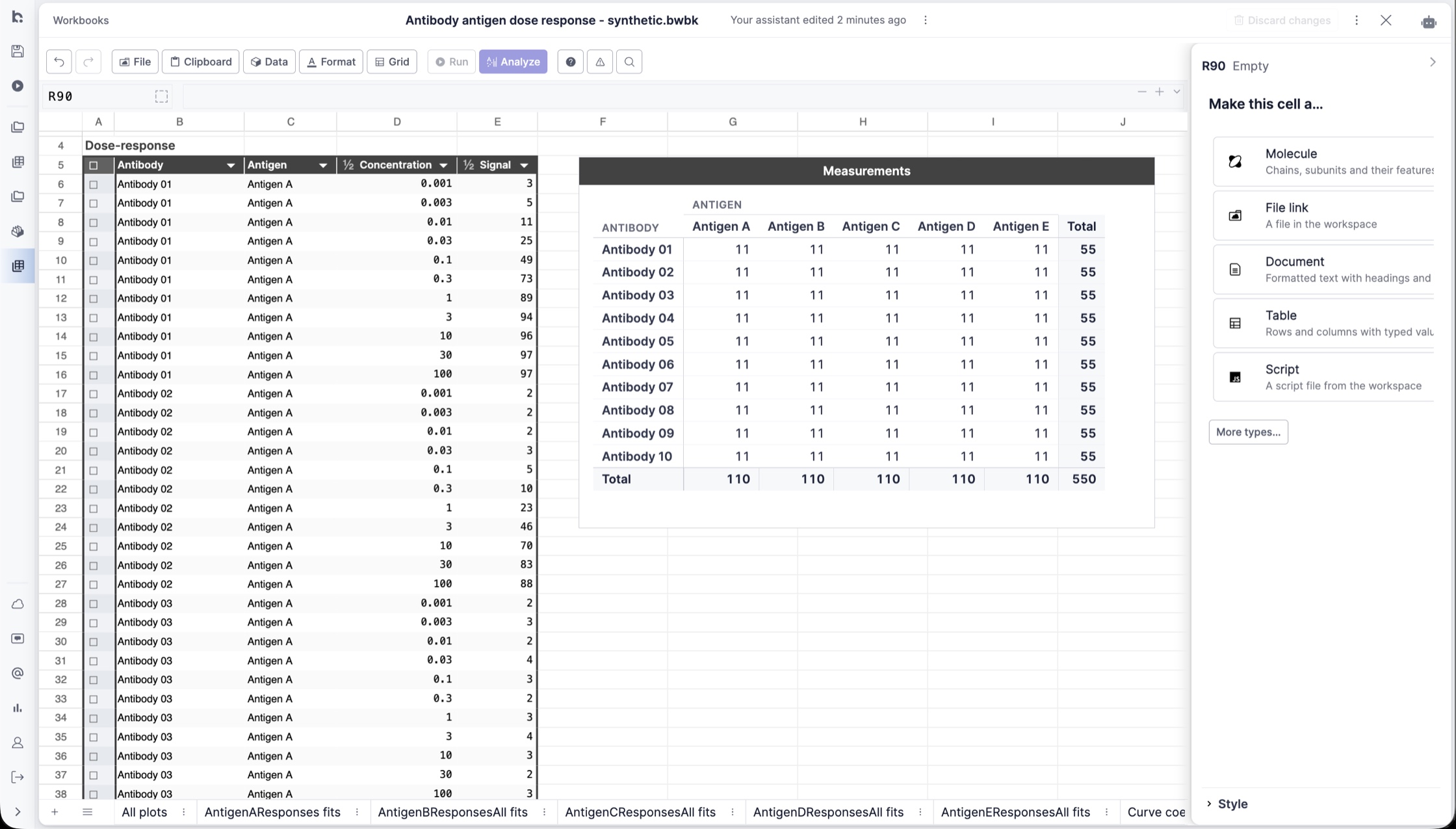
An assay export arrives in long form: one row per antibody, antigen, concentration and signal. In this example ten antibodies are titrated against five antigens over eleven concentrations, from 0.001 to 100 nM. A summary in the same workbook counts the measurements behind each antibody–antigen pair, so a short or duplicated series is visible before anything is fitted.
Fit every curve, and keep the ones that mean something
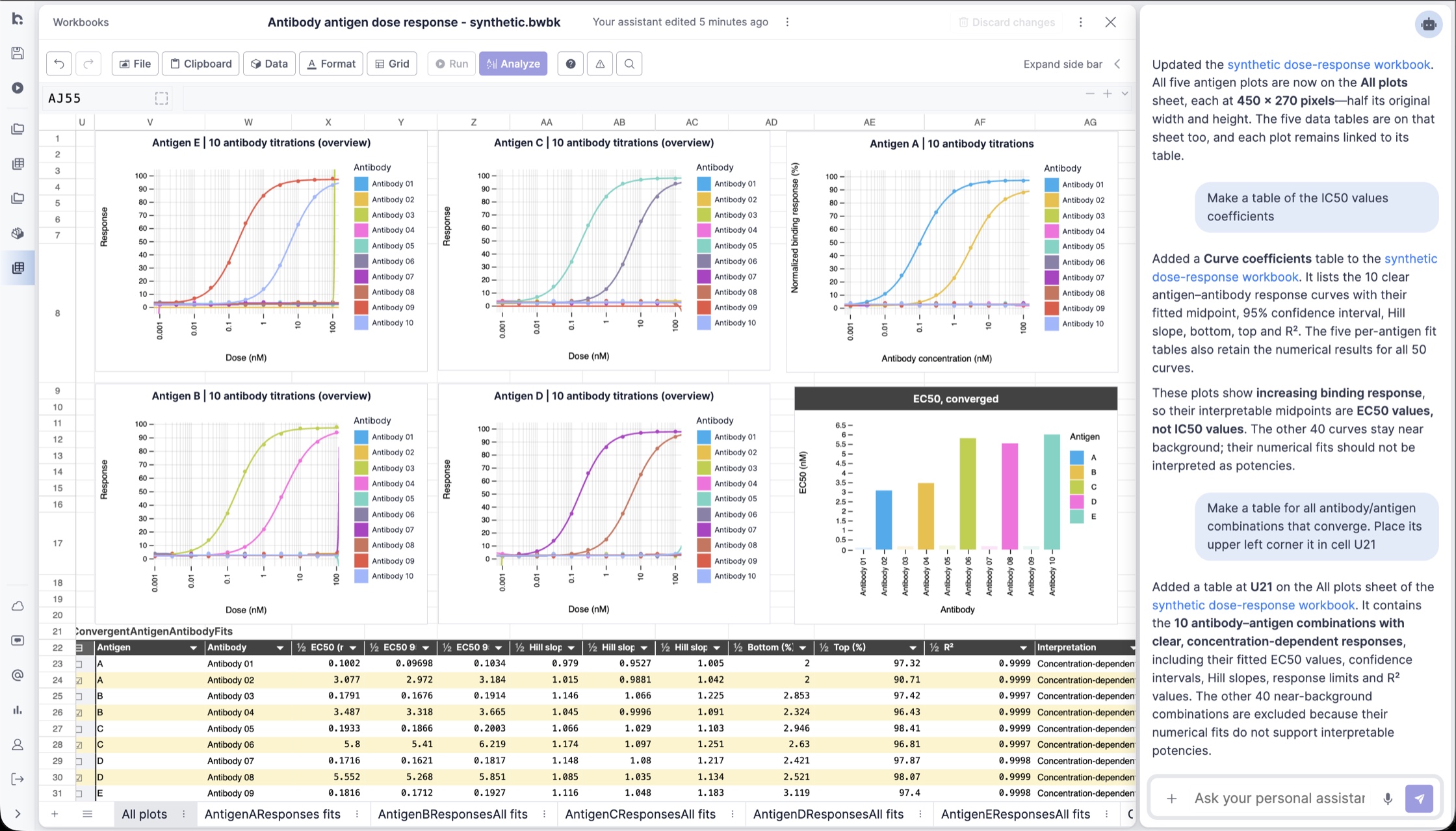
Each pair is fitted with a four-parameter curve for bottom, top, Hill slope and midpoint, and the fifty results are collected in one table with their confidence intervals and R². An overview plot per antigen draws all ten titrations together, so a responder reads against the background of the others.
Most of the panel does not respond, and the analysis says so. Ten of the fifty pairs give a clear concentration-dependent curve; the other forty stay near background and are excluded from the summary instead of being reported as potencies. The result is named correctly too: the signal rises with dose, so these midpoints are EC50 values, not IC50 values.
Customize the analysis
The curve model, the rule for what counts as a response, and the columns carried into the summary all live in the workbook, so a team can set them once and reuse the sheet for the next plate.